The Materials Data Science Book
Introduction to Data Mining, Machine Learning, and Data-Driven Predictions for Materials Science and Engineering
The Datasets Used Throughout the Book
The MDS book contains a large number of examples most of which require data in one or the other way. Interpreting results and debugging problems is easier if we have an intuitive understanding of the context of the dataset, e.g., with context we can answer whether 0.001 is a small number that can be neglected or whether it a significant value.
Therefore, a number of datasets with a materials science or physics background
are used. The book explains the materials scientific or physics background of
how the datasets were created as well as details of the datasets in
Chapter 4. The datasets can be openly obtained in
form of a Python package as described below.
Obtaining the Datasets
The datasets can be obtained in form of the Python package MDSdata
either using pip or directly from the GitHub repository.
It is recommended to install the package into a virtual Python environment.
A brief overview how this can be done is given here:
Creating and Using a Virtual Environment
It is advisable to use a virtual environment and install the Python
package there because then it is easier for python (i.e., for the
package manager "pip") to install all required dependencies
automatically in the correct version and to avoid conflicts with
other packages.
Here is a sketch of the most important steps for creating a virtual
environment in Linux using pyenv (no root permissions are
required):
- Install
pyenv: e.g., for Ubuntu/Debian-based systems this can be done in a terminal by running the code:
curl https://pyenv.run | bash
(see https://github.com/pyenv/pyenv-installer for more details). Most probably at the end of the installation you are reminded by the output in the terminal that you need to copy a few lines to the end of your .bashrc file. Read the terminal output carefully and if in doubt, check the above link for more information. -
Check the available Python versions:
pyenv install --list -
Install a particular Python version: e.g., python 3.9.7
pyenv install 3.9.7 -
Create a virtual environment and call it, e.g., "MDS" using the installed Python version:
pyenv virtualenv 3.9.7 MDS -
Activate the virtual environment with the name "MDS":
pyenv activate MDS -
To deactivate the virtual environment at the end and return to the system's default Python version, use:
pyenv deactivateYou can also simply close the terminal.
Note, that there are a number of different approaches to create and manage virtual environments, and the above is only one possibility.
Installing the Python package MDSdata
For this, there are mainly two options, for both of which it is useful to have created and activated a virtual environment, as explained above.- The recommended way: get the package directly from PyPI by running
pip install MDSdata
inside your terminal/virtual environment. - Alternative: Obtain the whole package from the
MDS data git repository.
After cloning or downloading the repository, change into it and then
inside the directory, install the package with
pip install .
(note the dot at the end). Make sure you run this command from within the repository at the same level wherepyproject.toml resides.
MDSdata
is available and can be used as detailed below.
Optional: Installing Jupyter Notebook
A convenient way of working with Python code is a
jupyter notebook. You can install this locally
into your virtual environment using
pip install jupyter
Afterwards, you can launch the juypter environment by running
jupyter-lab from your terminal.
Alternatively, you also can write your Python code with your preferred text editor
in a .py file and run it from the terminal with, e.g.,
python myfile.py.
For further information and instructions concerning the package, see the
How to Use the Datasets
With the above installation steps successfully finished, you are ready to either directly jumpy to one of the concrete examples for the datasets MDS-1...5 and DS-1 & 2 below or continue reading for getting some general information about the Python package.
Basic Steps and the two Interface Types to the Datasets
The name of the package is mdsdata (all lower characters!),
and you can just import it by import mdsdata. The
datasets are then directly contained in this namespace, e.g.,
mdsdata.MDS1 refers to the class MDS1 that contains
the data and some additional functionality for dataset MDS-1 (tensile test).
There are two ways of importing a specific dataset: for the most
flexibility use load_data, e.g.,
from mdsdata import DS2

images, labels = DS2().load_data(return_X_y=True)return_X_y=True returns the features and the target as
two numpy arrays, as_frame=True returns a pandas Dataframe,
and if no parameters are given a dictionary-like "Bunch" (in analogy to scikit-learn)
is returned that has the form
{data, target, taget_names, DESCR, feature_names}
A shorter alternative that chooses reasonable default values for the parameters
(and that therefore has less flexibility) is to use the
"named functions":
from mdsdata import load_Ising

images, labels = load_Ising()
As a shortcut, here is an overview of how to use the convenience wrapper around the classes for the MDS and DS datasets. This is (at least in the majority of all cases) the most easy to use approach:
TL;DR - Cheat Sheet for Loading the Datasets
| Dataset | Python Code for Importing the Dataset |
|---|---|
| MDS-1 tensile test |
|
| MDS-2 Ising microstructure |
|
| MDS-3 Cahn-Hilliard microstructure |
|
| MDS-4 Chemical elements |
|
| MDS-5 Nano- indentation |
|
| DS-1 Iris flowers |
|
| DS-2 MNIST digits |
|
| DS-2 (light) Alpaydin digits |
|
Materials Science Datasets MDS-1…5
Dataset MDS-1: Tensile Test with Parameter Uncertainties
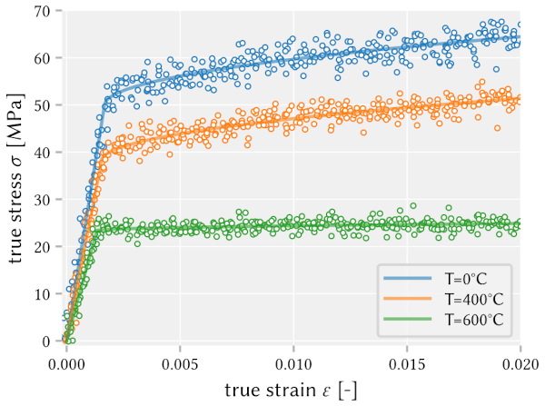
Summary: This dataset is obtained from simulating a linear elastic material model with non-linear hardening and temperature dependency.
Each data record was obtained using material properties that contain random contributions, mimicking uncertainties in the measurements. The solid lines show the average material response obtained for a set of mean material parameter values.
The dataset consists of the strain (the input or feature) and the stress (the output or target) for three different temperatures. It consists of altogether 350 data records for the strain covering 3 different temperature values (T=0°C, 400°C, and 600°C). For further details on the used equations and (material) parameters see section 4.2 of the book. In case that data for other temperature than those used in MDS-1 are needed, please take a look at the gitHub repository MDS-data and how MDS-1 is implemented.
Example: For how to obtain strain and stress data using the simple functions please see the above cheat sheet. The following lines of Python code import the dataset MDS1, store the data in six variables for stress and strain and then plot the data points:
import matplotlib.pyplot as plt
from mdsdata import MDS1
strain_T0, stress_T0 = MDS1.load_data(temperature=0, return_X_y=True)
strain_T400, stress_T400 = MDS1.load_data(temperature=400, return_X_y=True)
strain_T600, stress_T600 = MDS1.load_data(temperature=600, return_X_y=True)
fig, ax = plt.subplots()
ax.scatter(strain_T0, stress_T0, marker='.', label='T=0°C')
ax.scatter(strain_T400, stress_T400, marker='.', label='T=400°C')
ax.scatter(strain_T600, stress_T600, marker='.', label='T=600°C')
ax.legend()
plt.show()
strain_... and stress_... are 1D numpy arrays
and contain 350 elements each,
resulting approximately in the figure on the right.
If you prefer to use pandas DataFrame objects, you can obtain them
in the same way as also done in scikit-learn by setting the
parameter as_frame=True:
from mdsdata import MDS1
data = MDS1.load_data(temperature=600, as_frame=True)
display(data.frame)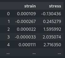
Here, load_data(...) returns a dictionary-like data "bunch" that
also contains a pandas DataFrame object.
The last command only works in a jupyter notebook and shows a formatted table with the output shown in the screenshot.
This is a good dataset for experiments with linear regression: you can either only use the elastic regime to fit a straight line, or you can use piecewise linear regression and treat the yield point as a hyper parameter. In the MDS book, this dataset is also used as an example for outlier detection.
Dataset MDS-2: Microstructure Evolution with the Ising Model
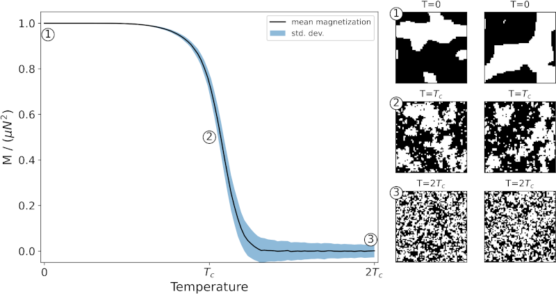
Summary: The Ising model is a statistical physics model used to represent, e.g., the evolution of ferromagnetic domain walls. Ernst Ising, to whom the model ows its name, was the first to solve it mathematically for a one-dimensional situation. The two-dimensional case is much more complex and here was solved numerically. The simulation method is based on the Metropolis Monte-Carlo method. After randomly initializing the system of, in our case 64 x 64 lattice sites (the pixels), its microstructure evolves. The figure shows some example microstructures. Each of them is characterized by a temperature which, in dimensionless scaling, is given as multiple of the so-called Curie temperature TC. The system undergoes a phase transformation at TC which shows in the transition from microstructures with strong fluctuations to microstructures with very distinct patterns.
In the MDS book, we use the Ising dataset, e.g., to explore the structure-property relationship: using a neural network we will predict the temperature (i.e., the property) based on the microstructural images. Furthermore, we investigate the data with the principle component analysis (PCA), and more advanced, embedding methods.
Example: The following lines of Python code import the dataset MDS2 using the simplified function and shows four example microstructures out of the altogether 5000 images:
import matplotlib.pyplot as plt
from mdsdata import load_Ising
images, labels, temperatures = load_Ising()
fig, (ax0, ax1) = plt.subplots(ncols=2, figsize=(8, 4))
ax0.imshow(images[10])
ax0.set(title=f"T={temperatures[10]:.2f}, label={labels[10]}")
ax1.imshow(images[3000])
ax1.set(title=f"T={temperatures[3000]:.2f}, label={labels[3000]}")
plt.show()
images is a 3D numpy array where the first index is the number of the image, e.g., in the above
example images[10] is the image number 10; temperature[10] is the temperature of that image, and label[10] is an integer value of 0 or 1, indicating if the temperature is below or above the Curie temperature.
Dataset MDS-2 (light): Ising Model, using small images
There is also a smaller Ising dataset that still contains 5000 images
which, however, are only 16x16 pixels in size.
It can be imported by from mdsdata import MDS2_light or for the simplified
interface by from mdsdata import load_Ising_light. Everything else stays the same as in MDS-2. Computations using this dataset are
considerably faster but lack some finer details.
Dataset MDS-3: Cahn-Hilliard Model
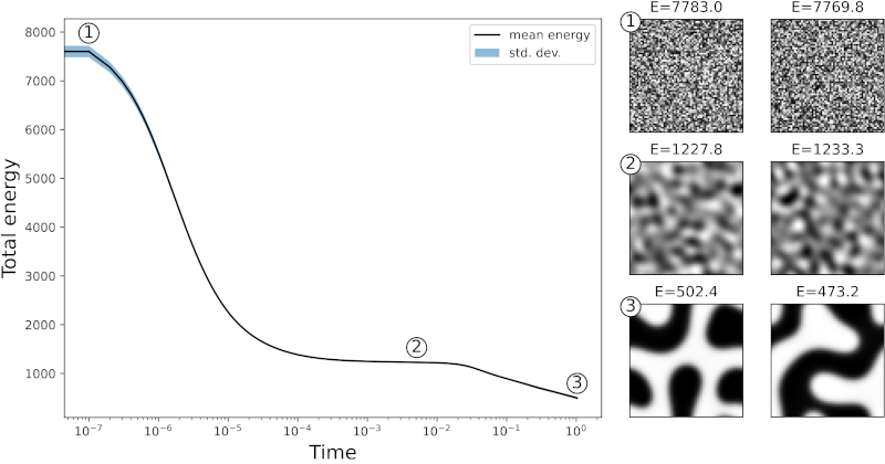
Summary: Binary mixtures, such as alloys of two metals, may coarsen into two phases, a mechanism which is described by the spinodal decomposition. This phenomenon may occur if an initially homogeneous phase becomes thermodynamically unstable. In this case, small fluctuations quickly grow.
In contrast to the Monte Carlo method used for creating dataset MDS-2 (Ising Model), there is no randomness in the evolution of this system; for given initial values, it is completely governed by continuum equations, i.e., the Cahn-Hilliard equation which were here solved by means of a finite element method.
The main "ingredients" for this model are the concentration of a phase, a free energy consisting of the potential, gradient, and elastic energy density. We are using such these datasets again for investigating the structure-property (=energy) relation but also in the context of unsupervised learning method and dimensionality reduction as well as for cross-validation purposes.
The dataset MDS-3 only contains data for a reduced energy range, as compared to the figure.
Example: The following lines of Python code import the dataset MDS3 consisting of data from altogether 17 simulations. It then shows some information, e.g., that the dataset consists of 17866 images of 64 x 64 pixel.
import matplotlib.pyplot as plt
from mdsdata import load_CahnHilliard
images, energies = load_CahnHilliard()
# or:
# from mdsdata import MDS3
# images, energies = MDS3.load_data(return_X_y=True)
print("The dataset contains", images.shape[0], "images.")
print("They are", images.shape[1], "x", images.shape[2], "pixel in size.")
print(f"The minimum energy is: {energies.min(): .1f}")
print(f"The maximum energy is: {energies.max(): .1f}")giving the following output:
The dataset contains 17866 images.
They are 64 x 64 pixel in size.
The minimum energy is: 457.7
The maximum energy is: 1099.8
The line containing MDS3.load_data(...) takes a few seconds
to run because the image data is contained
in an zip archive from which the images are extracted "on the fly".
A convenient way of using the dataset is in a juypter
notebook where this line with reading the data is only once executed at
the beginning of an experiment.
It is also possible to read data from a single simulation only which speeds
things considerably up. This is achieved by using, e.g., the parameter
simulation_number=3 which imports simulation number 3.
Dataset MDS-4: Properties of Chemical Elements
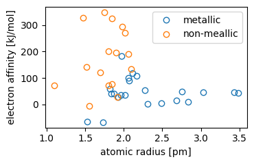
Summary: This is a small dataset that contains four periodic properties: atomic radius, electron affinity, ionization energy and the electronegativity. These properties were collected for a total of 38 chemical elements (22 metals and 16 non-metals), originally taken from a number of different publicly available sources.
The dataset can be used in the context of, e.g., supervised classification or unsupervised learning with methods such as clustering of data or principal component analysis. There, a simple task can be to decide, based on the chemical properties, if an element is a metal or not, or to find out, which are the most important periodic properties.
Example: The following lines of Python code import the dataset MDS4 and creates a scatter plot with two features, similar to the one shown above. The first code snipped uses the simplified function interface:
import matplotlib.pyplot as plt
from mdsdata import load_elements
atomic_radius, electron_affinity, \
    ionization_energy, electronegativity, label = load_elements()
fig, ax = plt.subplots()
ax.scatter(atomic_radius, electron_affinity, c=label)
ax.set(xlabel='atomic radius [pm]', ylabel='electron affinity [kJ/mol]')
plt.show()The second code snipped shows how to use the more general interface in analogy to scikit-learn and additionally shows a legend in the plot:
from mdsdata import MDS4
data = MDS4.load_data()
X = data.feature_matrix
label = data.target
features_names = data.feature_names
atomic_radius = X[:, features_names == 'atomic_radius']
electron_affinity = X[:, features_names == 'electron_affinity']
# Create array with True and False elements used for "filtering" metals/non-metals
# Note, that first, `label == 1` will be evaluated which is then assigned to `mask`
mask = label == 1
fig, ax = plt.subplots(figsize=(3.8, 2.5))
ax.scatter(atomic_radius[mask], electron_affinity[mask], c='C0', label='metallic')
ax.scatter(atomic_radius[~mask], electron_affinity[~mask], c='C1', label='non-metallic')
ax.set(xlabel='atomic radius [pm]', ylabel='electron affinity [kJ/mol]')
ax.legend()
plt.show()
To see all feature names you can use print(features_names).
If you prefer to use the Python package pandas then the following code
creates a DataFrame and additionally adds the text-label
for each value of the target variable:
# load the data and obtain the DataFrame object
chem_elem = MDS4.load_data(as_frame=True)
df = chem_elem.frame
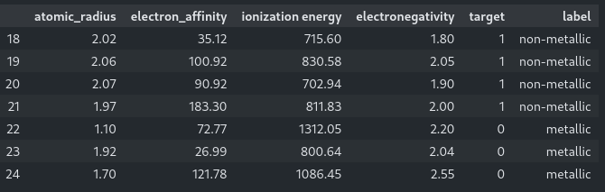
# include the text string labels for the 2 different classes of data:
df['label'] = df['target'].map(lambda i: chem_elem.target_names[i])
display(df[18:25])If run in a jupyter notebook the last command outputs the table from row 18 to row 24 where the newly created column showing the text string label can be seen:
Further details and references are given in section 4.6 of the MDS book.
Dataset MDS-5: Nanoindentation of a Cu-Cr Composite
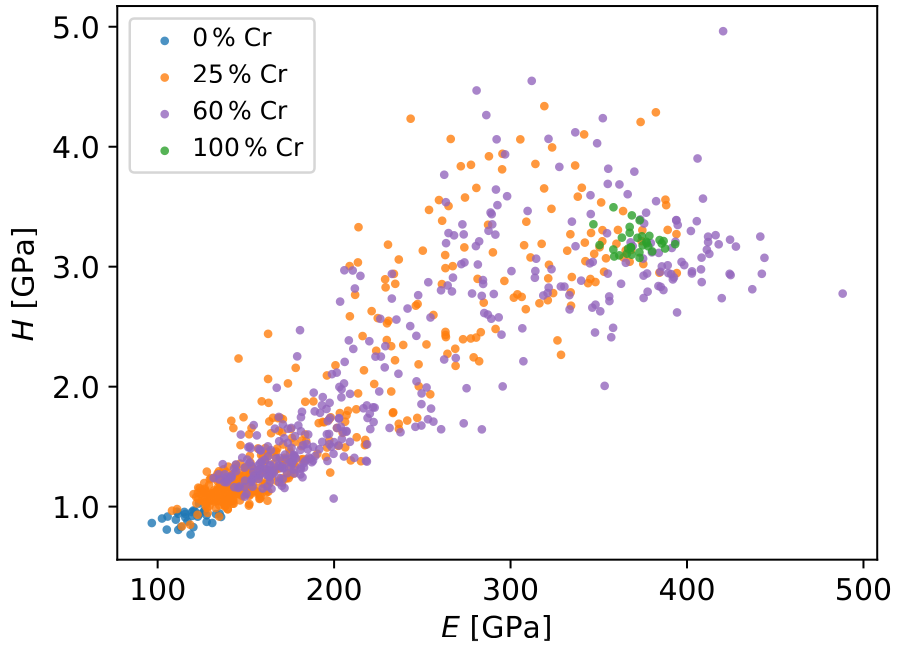
Summary: This dataset was obtained from nanoindentation of two different Cu-Cr composites containing 25 wt% Cr and 60 wt% Cr corresponding to 29.95 at% and 64.40 at% Cr, respectively. Additionally pure Cu and pure Cr datasets are contained that are used as reference data, covering the two extremes.
The dataset consists of two features: the hardness H and the Young's modulus E obtained for altogether 378 indents. Both are given in GPa. The four different material types are the class labels 0, ..., 3.
Example:
Calling the method MDS5.load_data() returns a dictionary-like object that contains the feature matrix data
consisting of modulus and hardness as the two features in columns.
The output "matrix" Y is a 1D array and contains for each
row an integer (0, 1, 2, or 3) that corresponds to the class_name
('0% Cr', '25% Cr', '60% Cr', or '100% Cr').
The following lines produce a plot similar to the figure shown above.
import matplotlib.pyplot as plt
from mdsdata import MDS5
CuCr = MDS5.load_data()
X = CuCr.feature_matrix
y = CuCr.target
print("The feature matrix has", X.shape[1], "features in columns:", CuCr.feature_names)
print(" ... and", X.shape[0], "data records as rows of X.")
print("The class labels 0...3 of Y correspond to:", CuCr.target_names)
modulus = X[:, 0]
hardness = X[:, 1]
material = y
fig, ax = plt.subplots()
ax.scatter(modulus, hardness, c=material)
ax.set(xlabel="Young's modulus [GPa]", ylabel="hardness [GPa]")
plt.show()
Setting c=material uses a different color for each of
the four different materials. The output of the print statements is
The feature matrix has 2 features in columns: ["Young's modulus", 'hardness']
... and 938 data records as rows of X.
The class labels 0...3 of Y correspond to: ['0% Cr', '25% Cr', '60% Cr', '100% Cr']
A second way of using the dataset is to only obtain the feature matrix and
the target data. This is achieved by specifying the return_X_y=True as in the scikit-learn library (see the docstring of the function for more details):
import matplotlib.pyplot as plt
from mdsdata import MDS5
X, y = MDS5.data(return_X_y=True, outlier=True)
plt.scatter(X[:, 0], X[:, 1], c=y)
plt.show()
Setting outlier=True has the effect that outliers are not
removed, which is useful for experimenting with methods for outlier
detections and removal. The default is that the postprocessed dataset with
outliers removed is returned.
“Classical” Datasets DS-1 and DS-2
Dataset DS-1: Iris Flower Dataset
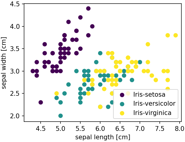
Summary: The Iris Flower dataset is one of the two most famous dataset used as "toy dataset" for first experiments with data science and machine learning.
The dataset contains the measurement of the length and width of two different types of leaves: the petals and the sepals, resulting in altogether 4 features. Additionally, the type of flower is contained: there are altogether 3 different Iris types, hence, the target variable can take the values 0, 1, or 3.
Example:
The following Python script shows how to load the dataset. Here we
use the mode general DS1.load_data() function (instead of load_iris())
as this gives us access to the names of the 3 class members.
For plotting the data of each class in a different color, we create an
array idx that acts as a "filter" (note that y == 2 returns an
array of boolean values, similar to np.where(y == 2, True, False)):
import matplotlib.pyplot as plt
from mdsdata import DS1
iris = DS1.load_data()
X = iris.data
y = iris.target
class_names = iris.target_names
fig, ax = plt.subplots(dpi=150)
idx = y == 0
ax.scatter(X[idx,0], X[idx,1], c=y[idx], label=class_names[0], vmin=0, vmax=2)
idx = y == 1
ax.scatter(X[idx,0], X[idx,1], c=y[idx], label=class_names[1], vmin=0, vmax=2)
idx = y == 2
ax.scatter(X[idx,0], X[idx,1], c=y[idx], label=class_names[2], vmin=0, vmax=2)
ax.set(xlabel='sepal length [cm]', ylabel='sepal width [cm]')
ax.legend()
plt.show()
The parameters vmin=0, vmax=2 are used to ensure that for each value
of y a unique color is chosen.
Clearly, the code could be written a bit more compact using a for loop.
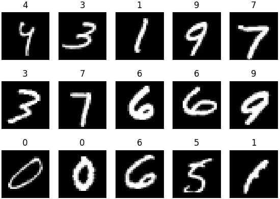
Dataset DS-2: The MNIST Handwritten Digits Dataset
Summary:
This is the famous MNST dataset of handwritten digits, a curated subset of a larger dataset collected by NIST. It contains 60,000 training images and 10,000 testing images of handwritten digits. The images are 28x28 pixels in size. The value range is 0 (background) to 255 (digit). Further information can be found at Yann LeCun's web page from which the dataset was obtained.
The dataset can be used for classification (the output of, e.g., a network is the integer value of the digit) but also for various "computer vision" problems, e.g., for denoising (when the digits are superimposed with noise) or impainting (i.e., "guessing" missing parts of such images).
Example:
Importing the MNIST dataset can be done in anaology to the above
datasets. The following example shows how to do this and additionally
creates a plot consisting of some randomly chosen images:
import matplotlib.pyplot as plt
import numpy as np
from mdsdata import load_MNIST_digits
rng = np.random.default_rng() # create a random number generator
# If you want to use the testing dataset instead use "train=False":
images, labels = load_MNIST_digits(train=True)
fig, axes = plt.subplots(ncols=5, nrows=3, figsize=(7, 5))
for ax in axes.ravel():
idx = rng.integers(low=0, high=images.shape[0])
ax.imshow(images[idx], cmap='gray', vmin=0, vmax=255)
ax.set(xticks=[], yticks=[], title=f"{labels[idx]}")
plt.show()
images array is the number of
the image such that images[12] gives the 13th image.
If the testing dataset should be used then the parameter train=False
needs to be set in DS2().load_data.
Showing a few stats of the dataset can be done as follows:
print("number of images:", images.shape[0])
print("number of images per digit: ", end='')
print(np.histogram(labels, np.arange(-0.5, 10.5, 1))[0])numpy's histogram function
to count the number of images
for each of the 10 classes (0..9). The [0] makes sure that only
the frequencies are printed and not the bin edges as well (the function returns
two arrays). The resulting output is:
number of images: 60000
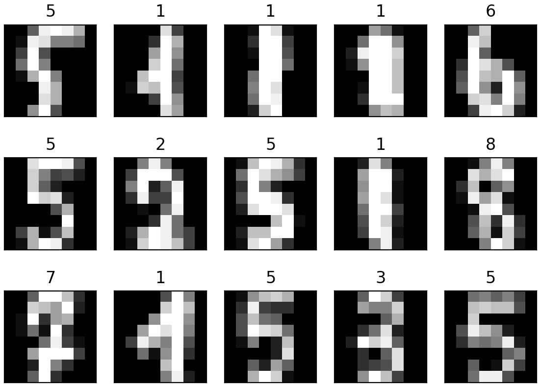
number of images per digit: [5923 6742 5958 6131 5842 5421 5918 6265 5851 5949]Dataset DS-2 (light): "Alpaydin" Handwritten Digits Dataset
Summary:
This is a smaller version of the famous MNST dataset of handwritten digits, prepared by E. Alpaydin. It contains 5,620 images of handwritten digits. The images are 8x8 pixels in size and were downsampled from the NIST dataset. The value range is 0 (background) to 255 (digit). Further information can be found in the UCI dataset archive from which the dataset was obtained.
The dataset can be used for classification (the output of, e.g., a network is the integer value of the digit) but also for various "computer vision" problems, e.g., for denoising (when the digits are superimposed with noise) or impainting (i.e., "guessing" missing parts of such images).
Example:
Importing the dataset can be done in anaology to the
MNIST
dataset. The following example shows how to do this and additionally
creates a plot consisting of some randomly chosen images:
import matplotlib.pyplot as plt
import numpy as np
# Variant 1: Loading the data
from mdsdata import DS2_light
images, labels = DS2_light().load_data(return_X_y=True)
# Variant 2: Loading the data
from mdsdata import load_Alpaydin_digits
images, labels = load_Alpaydin_digits()
rng = np.random.default_rng() # create a random number generator
fig, axes = plt.subplots(ncols=5, nrows=3, figsize=(7, 5))
for ax in axes.ravel():
idx = rng.integers(low=0, high=images.shape[0])
ax.imshow(images[idx], cmap='gray', vmin=0, vmax=255)
ax.set(xticks=[], yticks=[], title=f"{labels[idx]}")
plt.show()
images array is the number of
the image such that images[12] gives the 13th image.